12 Manage data with tidyverse
Let’s start with our first data analysis (I know you were waiting for it!): in this chapter, we will use the magic world of tidyverse and rnotebook to explore a dataset.
R notebook
We have already seen how to store R codes into scripts. However, there are some disadvantages of using them: you cannot see the output of a code directly under it, you cannot see the graphs directly under the code, you cannot create multiline comments without having to comment each line etc.Here comes notebooks! Whithin RStudio, just click “File” > “New File” > “R notebook” to open a new notebook.
As this book is not focused on it, and there is already a wonderful book about it, I invite you to read the first part of it to get used to this wonderful tool.
The key feature you need to understand are:
- code is executed only in code chunks, and all what you type outside is considered as “comment”
- after every executed code chunks you can see the output of the chunk itself (super useful for data visualization and dataframe inspection)
- you can export the notebook as html/pdf and share it with your colleagues (I prefer html for many reasons)
Dont’ worry! At the end of each chapter you can download the notebook used for the analysis, so you can explore it, see how it works, and run it. Don’t be lazy, first write your own notebook, in which you can add whatever comment you want, and then download mine to compare it.
Load packages and data
At the beginning of every analysis, it is strongly suggested to load any external package you want to use, in our case tidyverse. Why using tidyverse? Because it is super useful, easy to learn, intuitive and it is the main package used for data analysis with R. We have seen in the last chapter how to install and load it in our session, so let’s do it:
Next, we will load the dataset to analyze. It is taken from this paper, in particular it is Supplementary Table 13 (Download).
  SampleID Diagnosis Braak sex AOD PMI RIN CDR Area dataset
1 1005_TCX        AD     6   F  90   8 8.6  NA   TL    MAYO
2 1019_TCX        AD     6   F  86   4 7.8  NA   TL    MAYO
3 1029_TCX        AD     6   F  69   4 9.7  NA   TL    MAYO
4 1034_TCX        AD     6   F  88   5 8.9  NA   TL    MAYO
5 1045_TCX        AD     5   F  90  NA 8.4  NA   TL    MAYO
6 1046_TCX        AD     6   F  72   2 9.0  NA   TL    MAYO
Dataset structure
The very first thing to do is to explore the dataset, in particular the number of rows/columns and the type of columns. We can do it through str(), which returns the dimensions of the dataframe and some info about each column.
Here it is:
'data.frame':   1493 obs. of  10 variables:
 $ SampleID : chr  "1005_TCX" "1019_TCX" "1029_TCX" "1034_TCX" ...
 $ Diagnosis: chr  "AD" "AD" "AD" "AD" ...
 $ Braak    : num  6 6 6 6 5 6 5.5 6 6 5 ...
 $ sex      : chr  "F" "F" "F" "F" ...
 $ AOD      : num  90 86 69 88 90 72 85 82 77 90 ...
 $ PMI      : num  8 4 4 5 NA 2 NA 15 NA NA ...
 $ RIN      : num  8.6 7.8 9.7 8.9 8.4 9 8 10 8.6 7.9 ...
 $ CDR      : num  NA NA NA NA NA NA NA NA NA NA ...
 $ Area     : chr  "TL" "TL" "TL" "TL" ...
 $ dataset  : chr  "MAYO" "MAYO" "MAYO" "MAYO" ...
You usually know what data you have in your dataset, which variables etc. As this is a downloaded table and it is my first time looking at it, I have to admit that we have to discover few things ahahah
What can we say about this dataframe?
- It has 1493 observation and 10 variables
- Variable SampleID should be the unique identifier of the sample (we should check it)
- Diagnosis, sex, Area and dataset column can be categorical data, so we should convert them to factors
- We have NAs in some variables. I see your face asking yourself “What the hell are NAs?”. Don’t worry, we’ll explain it in a bit
Let’s now check if SampleID are unique identifiers; to do it, we evaluate whether the number of unique values in that column is equal to the number of total values of that column:
[1] TRUEYes, they are unique identifiers.
Change column type
Next, we transform some chr columns to factor, this has 2 main advantages: first of all, factors are treated differently in some functions (expecially plotting) and they occupy less memory in you PC.
“Factors?! Why are you telling me about this data type now?” Yes, this is another data type, but don’t worry, you just have to know the two advantages aforementioned and how to create it (we will see it now).
An you know what?! As I know you’re doing great, let’s introduce our first function of the magic tidyverse world: mutate:
df <- df %>%
  mutate("Diagnosis" = factor(Diagnosis),
         "sex" = factor(sex),
         "Area" = factor(Area),
         "dataset" = factor(dataset))

str(df)
'data.frame': 1493 obs. of 10 variables:
$ SampleID : chr "1005_TCX" "1019_TCX" "1029_TCX" "1034_TCX" ...
$ Diagnosis: Factor w/ 2 levels "AD","Control": 1 1 1 1 1 1 1 1 1 1 ...
$ Braak : num 6 6 6 6 5 6 5.5 6 6 5 ...
$ sex : Factor w/ 2 levels "F","M": 1 1 1 1 1 1 1 1 1 1 ...
$ AOD : num 90 86 69 88 90 72 85 82 77 90 ...
$ PMI : num 8 4 4 5 NA 2 NA 15 NA NA ...
$ RIN : num 8.6 7.8 9.7 8.9 8.4 9 8 10 8.6 7.9 ...
$ CDR : num NA NA NA NA NA NA NA NA NA NA ...
$ Area : Factor w/ 6 levels "BM10","BM22",..: 6 6 6 6 6 6 6 6 6 6 ...
$ dataset : Factor w/ 3 levels "MAYO","MSBB",..: 1 1 1 1 1 1 1 1 1 1 ...Great! It worked! Let’s dissect this code:
-
df <-: we reassign the result to the same variable (overwriting it) -
df %>%: this is a feature of purr, a package inside tidyverse, that takes what is at the left of%>%and pass it as the first input of the function after the symbol. We could have written this code in just one line, but in this way is more readable -
mutata(: we use the function mutate, with df as first input (implicit thanks to %>%). This function is used to create new column/s in the dataframe; if the column already exists (as in our case), it is overwritten -
"Diagnosis" = factor(Diagnosis)
: I take this as example, as this function has this structure -
factor(Diagnosis): it takes as input the column Diagnosis and transform it from chr to Factor
"new_column" = something. In this case, we create (overwrite) column Diagnosis with factor(Diagnosis). To note: in tidyverse functions, the column of the dataframe can be accessed by calling only the name of the column, and not df$name_of_the_column.
And what can we say about the result?
As you can see, the four columns we changed inside mutate has now changed their output: from chr they became Factor w/ n levels and a bunch of numbers instead of the values. I’m sure you have already understood what does it mean, but to be sure: with “levels”, R stores the unique values of that vector (remember, each column of a dataframe is a vector!), and then it uses, for each element, integers to refer to the corresponding levels. This ensure memory optimization (integers takes less memory/space than words).
But, don’t worry, when you ask R to visualize the values of a factor, it returns the value and not the numbers:
[1] AD AD AD AD AD
Levels: AD Control
Reorder levels of a factor
There is a cool feature about factors: you can order the levels of it. In fact, by default levels are in alphabetical order. We can see it here, using the function levels():
[1] "AD" "Control"Sometimes, it is useful to change the order of them: think about times (20 weeks comes before 3 days alphabetically), or having a control reference as first in plots (when plotting categorical variable, the order of the levels is the order in the plot).
So, let’s see how we can change the order of the levels using factor:
'data.frame':   1493 obs. of  10 variables:
 $ SampleID : chr  "1005_TCX" "1019_TCX" "1029_TCX" "1034_TCX" ...
 $ Diagnosis: Ord.factor w/ 2 levels "Control"<"AD": 2 2 2 2 2 2 2 2 2 2 ...
 $ Braak    : num  6 6 6 6 5 6 5.5 6 6 5 ...
 $ sex      : Factor w/ 2 levels "F","M": 1 1 1 1 1 1 1 1 1 1 ...
 $ AOD      : num  90 86 69 88 90 72 85 82 77 90 ...
 $ PMI      : num  8 4 4 5 NA 2 NA 15 NA NA ...
 $ RIN      : num  8.6 7.8 9.7 8.9 8.4 9 8 10 8.6 7.9 ...
 $ CDR      : num  NA NA NA NA NA NA NA NA NA NA ...
 $ Area     : Factor w/ 6 levels "BM10","BM22",..: 6 6 6 6 6 6 6 6 6 6 ...
 $ dataset  : Factor w/ 3 levels "MAYO","MSBB",..: 1 1 1 1 1 1 1 1 1 1 ...
“You are not using tidyverse now, why?” Right, I used the standard R syntax to highlight the syntax difference with tidyverse: in fact, here I had to put df$ into the function to explicit which column to convert. You can use whatever syntax you want, it does not matter at all; you will see shortly that sometimes tidyverse version is more clear.
Having said that, we can now see in the result of str() that now Diagnosis is an Ord.factor w/ 2 levels “Control”<“AD”.
Summary
Ok, now that we have fixed some columns, let’s evaluate the values of the dataframe, we will use summary():
   SampleID           Diagnosis       Braak       sex          AOD             PMI              RIN
 Length:1493        Control:626   Min.   :0.000   F:890   Min.   :53.00   Min.   : 1.000   Min.   : 1.00
 Class :character   AD     :867   1st Qu.:3.000   M:603   1st Qu.:79.00   1st Qu.: 3.917   1st Qu.: 5.60
 Mode  :character                 Median :4.000           Median :86.00   Median : 5.500   Median : 6.80
                                  Mean   :3.909           Mean   :83.59   Mean   : 7.471   Mean   : 6.67
                                  3rd Qu.:6.000           3rd Qu.:90.00   3rd Qu.: 9.167   3rd Qu.: 7.80
                                  Max.   :6.000           Max.   :90.00   Max.   :38.000   Max.   :10.00
                                  NA's   :97                              NA's   :45
      CDR           Area       dataset
 Min.   :0.000   BM10 :233   MAYO  :160
 1st Qu.:0.500   BM22 :238   MSBB  :930
 Median :2.000   BM36 :232   ROSMAP:403
 Mean   :2.368   BM44 :227
 3rd Qu.:4.000   DLPFC:403
 Max.   :5.000   TL   :160
 NA's   :563
How does summary works? It depends on the type of data of the column:
- Character: it returns the length and the class (See SampleID)
- Factor: it returns the number of occurrence of each levels (see Diagnosis, sex, Area and dataset). That’s another reason to use factor over character/numeric when possible. You can easily see if there are imbalance in some categories/levels or not.
- Numeric: it returns some descriptive (See Braak and others). As you should know the data types you have inserted, you know the range of values you are expecting, so this function helps you to immediately evaluate the presence of some outliers.
- Boolean: it returns the occurrence of TRUE and FALSE (as a factor with 2 levels)
Again, we have these NA’s… and now it’s the time to explain them.
Dealing with missing values
OPS, I already spoilered it ahahah. NA is the way R represent missing values.
In our example, we can see that we have different missing values in different columns, in particular in CDR where 1/3 of the total observations is missing.
How to deal with missing values is up to you. First of all, if you have collected the data it is a control on whether all your data are present (if not, you can go back and check why it is missing a data and fill it with a value, if you have it).
Usually, NA’s comes with downloaded data or data from different sources. You can decide if you want to delete all the observation with missing values, fill the missing values with another value (imputation) or accept missing values. There is not a standard on it, it is really up to you.
If you want to exclude all rows that have a missing value in any of the column, you should use na.omit function (I won’t show it because I don’t want to apply this filter to our data, but it is important that you know this function).
Instead, I propose an example on how to delete rows that have missing values in column PMI. We will use the function is.na() that evaluates values of a vector and returns a boolean (TRUE/FALSE) vector on whether a value is NA or not:
[1] FALSE TRUE TRUE FALSE FALSE FALSEYou should now tell me how to use it to exclude rows from a dataframe based on whether a value of a column is NA or not.
Here is you should have answered:
   SampleID           Diagnosis       Braak       sex          AOD             PMI              RIN
 Length:1448        Control:612   Min.   :0.000   F:864   Min.   :58.00   Min.   : 1.000   Min.   : 1.000
 Class :character   AD     :836   1st Qu.:3.000   M:584   1st Qu.:79.00   1st Qu.: 3.917   1st Qu.: 5.600
 Mode  :character                 Median :4.000           Median :86.00   Median : 5.500   Median : 6.700
                                  Mean   :3.881           Mean   :83.65   Mean   : 7.471   Mean   : 6.623
                                  3rd Qu.:6.000           3rd Qu.:90.00   3rd Qu.: 9.167   3rd Qu.: 7.800
                                  Max.   :6.000           Max.   :90.00   Max.   :38.000   Max.   :10.000
                                  NA's   :87
      CDR           Area       dataset
 Min.   :0.000   BM10 :233   MAYO  :117
 1st Qu.:0.500   BM22 :238   MSBB  :930
 Median :2.000   BM36 :232   ROSMAP:401
 Mean   :2.368   BM44 :227
 3rd Qu.:4.000   DLPFC:401
 Max.   :5.000   TL   :117
 NA's   :518
Great, we have no more NAs in PMI. If you don’t remember what ! stands for, go back and check the boolean chapter.
Filter a dataframe
We have just filtered out some rows, and guess what?! Tidyverse has a function to filter values, it is called…… filter.
This function takes as input an expression that returns a vector of boolean. Let’s try it to retrieve a dataframe of control males with CDR greater than 4:
df_male_ctrl_cdr4 <- df %>%
  filter(Diagnosis == "Control" & sex == "M" & CDR > 4)

summary(df_male_ctrl_cdr4)
SampleID Diagnosis Braak sex AOD PMI RIN CDR
Length:3 Control:3 Min. : NA F:0 Min. :89 Min. :2.667 Min. :4.900 Min. :5
Class :character AD :0 1st Qu.: NA M:3 1st Qu.:89 1st Qu.:2.667 1st Qu.:5.100 1st Qu.:5
Mode :character Median : NA Median :89 Median :2.667 Median :5.300 Median :5
Mean :NaN Mean :89 Mean :2.667 Mean :5.367 Mean :5
3rd Qu.: NA 3rd Qu.:89 3rd Qu.:2.667 3rd Qu.:5.600 3rd Qu.:5
Max. : NA Max. :89 Max. :2.667 Max. :5.900 Max. :5
NA's :3
Area dataset
BM10 :1 MAYO :0
BM22 :1 MSBB :3
BM36 :1 ROSMAP:0
BM44 :0
DLPFC:0
TL :0
We have just 3 observations that matches our request.
We can also use functions to evaluate thresholds etc. For example, let’s take the female whose RIN is above 3rd quartile (75th quantile):
df_female_rin3q <- df %>%
  filter(sex == "F" & RIN > quantile(df$RIN, p = 0.75))

summary(df_female_rin3q)
SampleID Diagnosis Braak sex AOD PMI RIN
Length:199 Control: 87 Min. :0.000 F:199 Min. :58.00 Min. : 1.000 Min. : 7.900
Class :character AD :112 1st Qu.:3.000 M: 0 1st Qu.:83.00 1st Qu.: 3.500 1st Qu.: 8.100
Mode :character Median :4.000 Median :88.00 Median : 4.750 Median : 8.500
Mean :3.899 Mean :85.07 Mean : 5.855 Mean : 8.708
3rd Qu.:5.000 3rd Qu.:90.00 3rd Qu.: 6.500 3rd Qu.: 9.200
Max. :6.000 Max. :90.00 Max. :30.000 Max. :10.000
NA's :10
CDR Area dataset
Min. :0.000 BM10 :13 MAYO :45
1st Qu.:0.500 BM22 : 9 MSBB :90
Median :2.000 BM36 :14 ROSMAP:64
Mean :1.978 BM44 :54
3rd Qu.:3.000 DLPFC:64
Max. :5.000 TL :45
NA's :109 There are 199 female samples with a RIN above 3rd quartile. We get it thanks to quantile function, which accept a vector and returns the quartile values; if you want a particular quantile (as in our case), you can give as input p, which is the quantile you want to calculate.
Sort for the value of a column
You can also sort the entire dataframe based on the values of a column (or more columns if ties are present). We do it through arrange function of tidyverse.
For example, let’s sort the dataframe based on RIN:
               SampleID Diagnosis Braak sex AOD       PMI RIN CDR Area dataset
1          hB_RNA_12624        AD     6   F  90  3.250000 1.0   4 BM10    MSBB
2          hB_RNA_12768        AD     6   M  82  6.833333 1.5   4 BM10    MSBB
3          hB_RNA_12695        AD     3   F  90  2.750000 1.8   3 BM10    MSBB
4           hB_RNA_8405        AD     5   F  85  9.166667 2.0   3 BM44    MSBB
5          hB_RNA_12615        AD     6   F  84  8.000000 2.1   3 BM10    MSBB
6          hB_RNA_10902        AD     5   F  73  7.333333 2.2   5 BM36    MSBB
7           hB_RNA_9005        AD     6   M  69  4.166667 2.2   5 BM44    MSBB
8          hB_RNA_10782        AD     5   F  90 11.833333 2.3   3 BM36    MSBB
9  hB_RNA_10782_L43C014        AD     5   F  90 11.833333 2.3   3 BM36    MSBB
10          hB_RNA_4341        AD     4   F  90  6.000000 2.4   4 BM44    MSBB
There are few consideration about this code:
-
We have sorted df based on RIN in an ascending order. If you want to sort the values in a descending way, you have to wrap the name of the column into
desc, asarrange(desc(RIN)) -
We piped (the symbol
%>%is also called pipe) the output ofarrangetoheadfunction, to get only top 10 rows to visualize -
Row 6 and 7 have the same RIN value, in this case we can add another column to
arrangeand use it to sort ties, asarrange(RIN, PMI)
Merge two columns
Sometimes, you want to merge two columns, and guess what?! There is a function for it ahahah
Let’s merge Area and dataset columns using unite():
  SampleID Diagnosis Braak sex AOD PMI  RIN CDR Area_dataset
1 1005_TCX        AD     6   F  90   8  8.6  NA      TL_MAYO
2 1019_TCX        AD     6   F  86   4  7.8  NA      TL_MAYO
3 1029_TCX        AD     6   F  69   4  9.7  NA      TL_MAYO
4 1034_TCX        AD     6   F  88   5  8.9  NA      TL_MAYO
6 1046_TCX        AD     6   F  72   2  9.0  NA      TL_MAYO
8 1085_TCX AD 6 F 82 15 10.0 NA TL_MAYOLooking at the code:
-
col =was used to set the new column name -
Area, datasetwere the two columns to merge. BUT, you can merge more than two columns, simply continue adding column names separated by a comma -
sep = "_"was used to set the separator between the values of the columns (in our case, the underscore) -
remove = Twas used to tell R to remove the columns that we have merged. If set to FALSE, the original columns are kept in the dataframe and the merged column is added
Split two columns
Obviously, there is also a function to split a column based on a patter: separate.
We use it to separate the newly created Area_dataset column into the original ones:
df <- df %>%
  separate(col = Area_dataset, into = c("Area", "dataset"), sep = "_", remove = F) %>%
  mutate("Area" = factor(Area),
         "dataset" = factor(dataset))

head(df)
SampleID Diagnosis Braak sex AOD PMI RIN CDR Area_dataset Area dataset
1 1005_TCX AD 6 F 90 8 8.6 NA TL_MAYO TL MAYO
2 1019_TCX AD 6 F 86 4 7.8 NA TL_MAYO TL MAYO
3 1029_TCX AD 6 F 69 4 9.7 NA TL_MAYO TL MAYO
4 1034_TCX AD 6 F 88 5 8.9 NA TL_MAYO TL MAYO
6 1046_TCX AD 6 F 72 2 9.0 NA TL_MAYO TL MAYO
8 1085_TCX AD 6 F 82 15 10.0 NA TL_MAYO TL MAYOHere it is! We have regained the original columns as well as the merged one.
As you may have guessed, into = is used to set the names of the columns that are created by this function.
Merge two dataframes
To conclude this chapter, we will see how to merge two dataframes based on the values of a common column.
This is useful when, for example, you have the output of a differential gene expression with ensemble gene id and another dataframe which associates the ensemble gene ids with gene names, chromosome position etc etc. In this way, you can bring the information of the second dataframe into the first one.
In our case, I found in the paper the extended names of the Area abbreviations, and I want to add this info to our table. To do so, let’s first create the dataframe of abbreviations and full names:
# 1. Create vectors
abbreviations <- c("BM10", "BM22", "BM36", "BM44", "DLPFC", "TL")
full_name <- c("Broadmann area 10", "Broadmann area 22", "Broadmann area 36", "Broadmann area 44",  "Dorsolateral prefronal cortex", "Temporal lobe")

# 2. Create dataframe
area_df <- data.frame(abbreviations, full_name)

area_df
abbreviations full_name
1 BM10 Broadmann area 10
2 BM22 Broadmann area 22
3 BM36 Broadmann area 36
4 BM44 Broadmann area 44
5 DLPFC Dorsolateral prefronal cortex
6 TL Temporal lobeNext, to insert full_name info into our original dataframe we have to use one of the join functions from dplyr package of the tidyverse universe:
  SampleID Diagnosis Braak sex AOD PMI  RIN CDR Area_dataset Area dataset     full_name
1 1005_TCX        AD     6   F  90   8  8.6  NA      TL_MAYO   TL    MAYO Temporal lobe
2 1019_TCX        AD     6   F  86   4  7.8  NA      TL_MAYO   TL    MAYO Temporal lobe
3 1029_TCX        AD     6   F  69   4  9.7  NA      TL_MAYO   TL    MAYO Temporal lobe
4 1034_TCX        AD     6   F  88   5  8.9  NA      TL_MAYO   TL    MAYO Temporal lobe
5 1046_TCX        AD     6   F  72   2  9.0  NA      TL_MAYO   TL    MAYO Temporal lobe
6 1085_TCX        AD     6   F  82  15 10.0  NA      TL_MAYO   TL    MAYO Temporal lobe
Just a couple of comments on the code:
-
y =is used to set the dataframe that has to be joined -
by =is used to declare which variable of the first dataframe is to match in the second dataframe (in our case Area from the first with abbreviations in the second) -
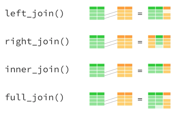
There are many join functions:
-
left_join(the one we used): keep all the rows of the first dataframe, even if there is not the correspondence in the second on, and only the rows of the second one that have a match in the first -
right_join: keep all the rows of the second dataframe, even if there is not the correspondence in the first one, and only the rows of the first one that have a match in the second -
inner_join: keep only the rows that have common values between the two dataframe in the column used to merge -
full_join: keep every rows of both dataframes
-
This concept is easier to explain with this image:
Exercises
Woah… this was tough. Let’s do some exercises to strengthen these concepts.
Exercise 12.1 The first exercise is not a practical exercise sorry… I want you to read this very short paper on how to structure tabular data. I is mainly on Excel (which you know… NEVER use it anymore to do analysis), but the key concepts must be applied to every tabular data you are creating.
Next, take one of your data file from an experiment and try to be consistent with what you have just read.
Exercise 12.2 Take our dataset and filter for males samples of Temporal lobe and female samples of Dorsolateral prefronal cortex.
Change full_name to a factor
Solution
df_filtered <- df %>%
  filter((sex == "M" & full_name == "Temporal lobe") |
           (sex == "F" & full_name == "Dorsolateral prefronal cortex")) %>%
  mutate("full_name" = factor(full_name))

summary(df_filtered)
SampleID Diagnosis Braak sex AOD PMI RIN
Length:318 Control:152 Min. :0.000 F:263 Min. :61.00 Min. : 1.000 Min. : 5.000
Class :character AD :166 1st Qu.:3.000 M: 55 1st Qu.:84.45 1st Qu.: 4.021 1st Qu.: 6.500
Mode :character Median :4.000 Median :89.20 Median : 5.375 Median : 7.400
Mean :3.751 Mean :86.37 Mean : 7.143 Mean : 7.271
3rd Qu.:5.000 3rd Qu.:90.00 3rd Qu.: 8.167 3rd Qu.: 8.000
Max. :6.000 Max. :90.00 Max. :33.000 Max. :10.000
NA's :25
CDR Area_dataset Area dataset full_name
Min. : NA Length:318 Length:318 MAYO : 55 Dorsolateral prefronal cortex:263
1st Qu.: NA Class :character Class :character MSBB : 0 Temporal lobe : 55
Median : NA Mode :character Mode :character ROSMAP:263
Mean :NaN
3rd Qu.: NA
Max. : NA
NA's :318
This was just an introduction with some cool stuff you can do with tidyverse. In the next chapter we will see more functions that can help us in doing statistics and other useful operations.